Background modeling via spline gradient descent optimization

The problem

Some of the light we capture does not come from the object we are photographing. Moonglow, airglow, and, unfortunately, light pollution, get all the way to our pixels. These 'background' light sources are unwanted and they get mixed unavoidably with our object signal. 

Essentially we are assuming that our image can be decomposed as the sum (or maybe the multiplication) of an object term and a sky background term. If we compute an estimation of the second, we can recover to some extent the object term by subtracting the background estimation from the original image.

There is no way to tell what part of the signal comes from the object and what comes from the contribution of the sky background. In this sense, this is an ill-posed problem. In order to face it, we establish the hypothesis that the background contribution should be a "pretty smooth" gradient. From that, we need some way to compute a model, that is, an estimation, of the sky background. 

Existing solutions

There are essentially two different processes to do this: in PixInsight, they are named "Automatic Background Estimation" and "Dynamic Background Estimation", or ABE and DBE, for short. 

ABE uses a polynomial model of an arbitrary degree for the generation of the background. Polynomials with lower degrees are very smooth and can handle very well slowly varying gradients, usually found in relatively longer focal lengths. Higher degrees lead very easily to oscillation and should therefore be avoided in general. To compute the sky background, we need to fit the polynomial model to our existing image by sampling the background. How do we do this? These samples should be representative of the background signal. ABE places the samples automatically using a grid pattern, and then evaluates statistically their background representativeness based on some user-provided parameters, weighting every sample. 

DBE, in contrast, lets the user place the samples manually (in this sense "dynamic" can be interpreted as "interactive"). So we are responsible of picking the best spots for the samples, that is, the small areas where we estimate visually that only sky background is present. As previously said, there is no way we can tell that, but doing some exploratory analysis (i.e., a heavy stretch of the left side of histogram over a copy of the original image, where we optionally could have applied previously a smooth ABE subtraction to make background areas more evident) we may generally have a solid clue. Moreover, the sampling method used by DBE, like ABE, also statistically weights every sample so they are robust to outliers. DBE uses a spline-based model, so it produces very smooth gradients that do not tend to oscillate as high-order polynomials do. Usually, just 2-order splines are enough to find a good background estimation. 

As we suppose that the background gradient is smooth, both tools usually work on a downscaled copy of the image, to speed up computations. 

So we have an automatic tool that works well for simple gradients and a very powerful tool that fits very well more complex gradients, but needs the user's eyes to distinguish what is what (background only vs background and object signal). 

The background extraction process should be applied early on our workflow, usually on the integrated master frames, still in linear phase. It could also be extracted on every calibrated light subexposure, but the computational cost would be high; instead, when the gradients vary significantly among exposures, what we usually do is normalize them just before integration (see Adaptive Normalization in ImageIntegration or the NormalizedScaleGradients script documentation), something that makes pixel/outlier rejection more effective, and after integration, the residual gradient is removed by background extraction. 

Proposed Approach

First, this approach is not a substitute for the ABE or DBE tools. As usual in data science, it is just another tool in the box, that may fit better or worse than the other for a particular image. 

Having that in mind, our goal here is creating a tool that has the modeling power of DBE, i.e. based on 2D-splines, and the automatic sampling feature of ABE. For this approach we will be using a typical machine learning optimization tool: a gradient-descent algorithm. We need a goal to optimize for, something that in machine learning turns into defining a loss function that the gradient descent will minimize, iteratively. In this regard, note that "gradient"(-descent) refers to the gradient of the loss function, not the background gradient that is blended in our image. This algorithm will be computationally intensive as it has to compute a 2D-spline in every iteration to evaluate the loss function. That's what we trade here: manual intervention for heavy computation. To alleviate this to some extent, though, and limit the memory use, we will be also working on a downscaled version of the original image, as ABE and DBE do. By default, downscaling is done by computing the median value of each block, so most small stars get filtered out. 

In this way, the problem to solve becomes the selection of the loss function. As usual in machine learning, the loss function will be a composition of several terms, in this case combined by a simple addition:

• reconstruction or "error" term: measures the difference between the background estimation and the image, so we try to "inflate" the background estimation as much as we can;
• "overshoot" term: penalizes if the background estimation becomes brighter than the image itself in some areas to avoid "inflating" it too much;
• "negative" term: additional penalty if the background estimation has negative values;
• color balance term: only meaningful if the image has RGB channels, it measures the variance among channels, trying to avoid color casts in areas where the background estimation could be slightly more aggressive on one channel than the others. 

The overshoot and negative terms are weighted by the 'alpha' parameter, to experiment with their effect. 

The gradient descent algorithm updates the parameters that define the 2D-spline in each iteration. These parameters include the position of the samples and a set of weights for the basis functions of the spline. The initialization of the algorithm, which is stochastic in nature, is essential for finding a good solution in a reasonable time. In this case, initial sample placement can be random or grid-based, and the initial sample values are the image pixel values where the samples are placed. 

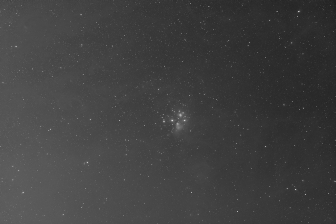Input image (M45 widefield). Stretched for visualization. 

Background-subtracted image on each iteration of the gradient descent algorithm (stretch based on the last image). 

Background model estimated with bgoptimizer (stretched). 

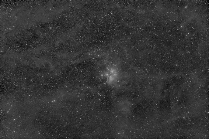Output image (stretched). 

On images where bright, relatively large regions exist it may be convenient to mask them so the initial spline will not be locally biased towards them. Masking has two effects on the algorithm: in the initialization, masked pixels' values are blended with the overall median value of the image (an overall background estimator); during the optimization, masked positions are not included in the loss function evaluation. Note that this does not mean that sample positions that lie on masked pixels are ignored: all of them, and their associated basis function weights, are used to calculate the spline. 

Masking could also be effective for ignoring areas like a landscape. By default, missing values (e.g., "black" regions resulting from registration) are also masked. Of course, the mask values can also be anywhere between 0 and 1, to modulate their effect. 

Original skyscape image (actually a sequence registered and integrated for the sky). Stretched for visualization.

Background-subtracted skyscape image, after masking the landscape (stretched).

There is also an important matter regarding the input image: the loss function needs proper scaling of the relevant data, i.e., the background itself. So, to correctly preprocess a linear image, the first step involves a non-linear stretch that should:

• reveal the faint structures over the background as much as possible;
• be reversible, so the computed background estimation can be mapped back to a linear state, making its value range compatible with the input image.

Once the background model has been fitted, the process generates a full-resolution version of the background estimation, reverses the preprocessing steps to make it linear, and subtracts it from the original image. 

Implementation

The provided implementation is written in Python, using Keras/Tensorflow packages, so it can take advantage of systems with GPU. The optimization process is implemented as a regular deep learning model built on a custom Spline layer. This layer uses internally _solve_interpolation() and _apply_interpolation() from the tfa.image.interpolate_spline module (as of TF 2.5 anyway) [1]. Note that these methods are accesible but not really public so this (unfortunately) means that changes in the internal implementation of tfa.image.interpolate_spline may lead to a rewrite of the Spline layer. 

The preprocessing step over the input image, in linear stage, is implemented by applying a Midtones Transfer Function or MTF (actually a slight variation of the MTF as defined in the XISF specification [2]) that delinearizes the image, along with a scaling based on a user-specified quantile to reveal the faint signal. This scaling usually saturates the brightest parts of the image, but takes into account that we are interested in optimizing the background, and we can ignore those highlights by masking them (usually even a simple threshold-based mask could suffice in many situations). 

The implementation is provided as a command line script. The description of each parameter is described on the repository page, along with some usage guidelines. A Google Colab notebook is also provided to test the process using your images without the need of a locally installed Python environment. See the Download section below. 

It only accepts XISF files, using the xisf package, to avoid format conversion in my PixInsight workflow. 

Future work

Needs more testing, and probably adjusting loss terms. A new term to penalize spline complexity has been explored, but it seems that simply with the spline order parameter it can be sufficiently controlled. The color balance term in particular has not been tested much. 

Also, using the global median value as initial values for samples in masked regions is disputable. Should we apply the mask to the image in order to compute the global median? This also requires experimentation.

The current implementations relies heavily on _apply_interpolation() function of Tensorflow addons, which evaluates the spline in each pixel for every iteration. This function needs an array of the pixel positions to evaluate: As in this case every pixel is evaluated, maybe a different implementation of this interpolation could use less memory. Another option would be to exclude fully masked pixels from the array, as they are not evaluated in the loss function anyway. However, the interpolation of the full resolution background estimation should include all pixels. 

From the deployment perspective, more work is needed in other areas to facilitate it, e.g. by providing binaries without external dependencies and to better integrate it with PixInsight by a custom PJSR script. Ideally, the stretching parameters should be interactively adjustable on the script using a preview of the image. 

References

[1] Tensorflow 2 documentation. tfa.image.interpolate_spline.

[2] J. Conejero. XISF Version 1.0 Specification. 2017.

 

Download

bgoptimizer